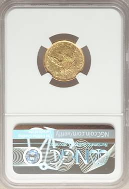
The 1881-O is the rarest New Orleans Mint eagle from the early part of this decade. Coins graded AU55 to AU58 are very rare, and there are only a small number of Mint State examples known. In 2006, Winter reported probably four of five Uncirculated pieces extant, a number that likely hasn’t changed appreciably, despite inflated certification totals. This one is semi-prooflike and quite flashy in its appearance. Tied with 7 others for the highest graded by NGC.
Offered at $21,275 delivered
We do business the old fashioned way, we speak with you.
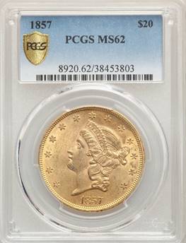
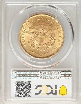
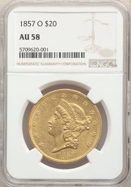
The 1857 Liberty double eagle claims a mintage of 439,375 pieces and the issue is not difficult to locate in circulated grades up to the XF-AU level. This issue was not nearly as well-represented in recent shipwreck finds as its San Francisco counterpart, with only two examples recovered from the S.S. Central America and 26 found in the wreck of the S.S. Republic. As a result, the 1857 is rare in MS62 condition, and a prime condition rarity in higher grades. The one offered here displays a crusty area at approximately 1:00-2:00 at the obverse rim. We prefer to leave it as is, for its originality. The PCGS population is just 28 with 7 higher.
Offered at $17,250 delivered
We do business the old fashioned way, we speak with you.
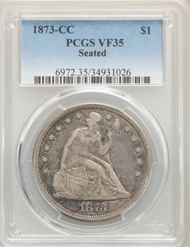
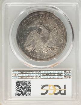
Struck to the extent of a meager 2,300 pieces, the 1873-CC Seated dollar melds the perennial popularity of the Carson City Mint’s CC mintmark with the last year of issue for the Seated dollar design into an in-demand numismatic rarity. The paltry surviving population was further reduced by the likely melting of a large majority of the coinage in April 1873 at the Carson City Mint. Circulated examples in any grade are rare, and Mint State pieces are among the proverbial numismatic hen’s teeth. PCGS has graded only 95 pieces (including re-submissions) in all grades combined.
Offered at $22,715 delivered
We do business the old fashioned way, we speak with you.
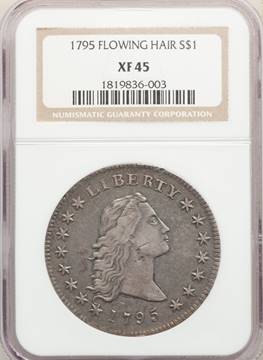
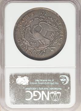
Flowing Hair Dollars were struck for less than two years before their replacement by the longer-lived Draped Bust type. High-grade survivors of this brief series are under tremendous demand from type set collectors. Unlike so many others and thankfully, this one looks un-dipped/original and displays even medium steel-grey color on both obverse and reverse.
Offered at $9,200 delivered
We do business the old fashioned way, we speak with you.
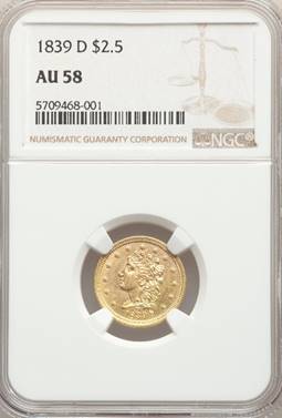
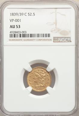
The Dahlonega Mint opened for business in 1838, for the purpose of providing a coinage facility for miners of Southern gold and to service the local economy. As a result, coins produced at the Georgia branch mint circulated extensively. The first gold pieces struck at the Dahlonega Mint in 1838 were half eagles. Quarter eagles followed in 1839. In both cases, the first-year issue is a one-year type showing William Kneass’s Classic Head Liberty design. The NGC population is just 18 with 14 higher.
Offered at $15,525 delivered
We do business the old fashioned way, we speak with you.
Authored by Curvature Securities‘ Scott E.D. Skyrm, one of the world’s most-respected repo market participants and experts. 10/08/2019 – 15:28
Panic At The Repo
As a professional trader, I keep an eye out for the next panic or market crisis. Since the beginning of my career, there was a crash or panic every few years in one market or another. You try to think about what market is overbought. What market is in a bubble. What market just appeared on the cover of Time Magazine! Little did I ever imagine the Repo market would experience the next big panic. This is a market consisting of AAA-rated risk-free securities backed by the United States of America! How can there be a crisis in U.S. Treasury securities? We didn’t even make the cover of Time Magazine!
I write about the Repo market every day. As a service to our clients, I decided to put everything I know about the Repo market collapse down on paper. So here it is!
Modern Day Bank Run
We’ve seen the old pictures or films of people lining up outside of a bank to collect their deposits. Think of the Depression in the 1930s. Knowing that a bank can’t make good on all of their customers’ deposits means the first people to get their money are more likely to get their money. Period. Banks never keep all of their customers’ deposits as cash on hand. They invest those customers’ deposits by making loans – like a mortgage loan to a family to buy a home or loan to a business to help start a new venture. Banks invest in loans and borrow money through deposits. That also means they loan long-term and borrow short-term. Don’t worry, this is important later on.
Though banks still have the same problem today – lending long-term and borrowing short-term, increased regulation and stronger risk management has forced them to narrow the tenure mismatch. These days banks have a larger percentage of their funding borrowed in the term markets by issuing CDs, medium-term notes, and even bonds. Since banks manage their tenure mismatch much better, they are not as susceptible to the classic “run on the bank.” However, in recent years, new categories of financial institutions have popped-up that are more susceptible to “bank runs.”
Shadow Banking
The term “shadow banking” is often thrown around as the perennial risk to the financial system. There is no real definition of a “shadow bank,” but they are a key part of the Repo market and the Repo market made “shadow banking” possible. Basically, a “shadow bank” is a financial institution that performs banking functions. A “shadow bank” can be anything from a REIT (Real Estate Investment Trust), to a mortgage finance company, to a hedge fund, to a broker-dealer (like MF Global). The easiest example is a mortgage REIT. They buy mortgage-backed securities (MBS), basically mortgage loans that were packaged into securities, and borrow money to finance those securities in the Repo market. Comparing the REIT to a bank, the REIT’s “loans” are the mortgage-backed securities and the Repo transactions are the “deposits.”
Just like a bank, the REIT’s MBS portfolio might have an average weighted maturity of, say, 7 years. Their Repo transactions might be anywhere from overnight to three months. In this simple example, the REIT is lending 7 years and borrowing between overnight and three months. This maturity mismatch problem exists for “shadow banks” just like it exists for regular banks. But there is no regulation that forces “shadow banks” to mind their mismatch. As I said, this is all important later on.
Crisis of Too Few Securities
Maybe the whole Repo crisis really began several years ago. Yes! Blame it on the Financial Crisis. Just a few years ago, the Fed was in Quantitative Easing mode and buying Treasury and agency MBS securities, thus removing them from the market. At the time, I called it a back-door method to finance the budget deficit; but it worked. The combination of bond purchases and a fed funds target range of 0.0% to .25% pushed GC Repo rates close to zero. With rates set so low and the Fed still buying $50 billion of securities every month, Treasury securities were becoming scarce in the Repo market. By July 2013 QE purchases had taken so many Treasurys out of the market that the Fed was left with a SOMA portfolio of over $4 trillion. At this point, GC Repo rates were close to zero. If overnight rates turned negative, there would be tremendous stress on the Repo market, money market funds, and the Treasury market overall.
In the blink of an eye, the Fed announced the Reverse-Repurchase Program as a facility to put securities back into the market. And they rolled out this program very quickly. Announcing it in August 2013 and beginning operations in September 2013. Approved participants (not just Primary Dealers) could submit their cash to the Fed and receive Treasury securities in exchange as collateral. The perfect solution to a shortage of collateral. Cash investors, like money market funds, immediately found a new counterparty to invest their cash. They could trade with the AAA-rated Federal Reserve and receive AAArated U.S. Treasury securities. Not a bad deal! You can’t get any more risk free than that!
Pressure Building
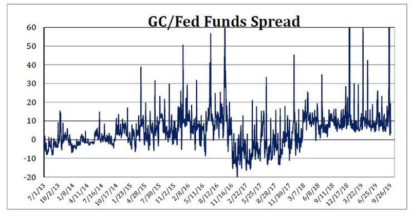
Between 2013 and the present day, a lot of things changed. The Treasury kept issuing more and more debt to fund the budget deficit, thus putting more and more Treasury securities into the market. The Federal Reserve began the QE “runoff,” where they stopped reinvesting the principal and interest of maturing SOMA portfolio securities. This put upward pressure on GC Repo rates and the spread between GC Repo and fed funds began to increase. Whereas GC Repo rates were averaging about 5 basis points below fed funds in July 2013, they now average about 10 bps above fed funds. That’s a large move!
Bank Reserves
While more and more collateral was accumulating in the Repo market, bank reserves were dwindling. Banks are required to hold a certain percentage of their liabilities in cash. This cash can be delivered to a special account at the Federal Reserve and the Fed will pay the banks an interest rate on their cash/reserves. What’s more, if banks have extra cash, they can deposit that cash at the Fed and the Fed will pay them interest on their “excess reserves.” That’s the Interest On Excess Reserves (IOER) rate. But the key point is that banks choose to leave excess reserves at the Fed. If there is a better short-term investment, they are allowed to remove that cash and invest it elsewhere.
Total bank reserve balances peaked at around $2.8 trillion in 2014 and have slowly declined since then. These days, those reserves are down to about $1.7 trillion. Yes, there’s been a significant decline, but nothing off trend in 2019, let alone no significant changes in
September 2019.
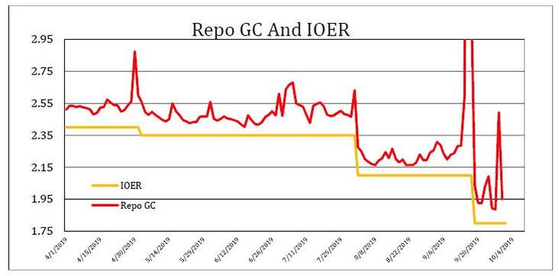
The Fed had been cut ting the IOER all year long. At the beginning of 2018, the IOER was set at the upper end of the fed funds target range. Since then, when the FOMC either raised or cut the fed funds target range, they often raised the IOER less than 25 basis points with a tightening or lowered the IOER more than 25 basis points with an ease. Since the September FOMC meeting, the fed funds target range was lowered to 1.75% to 2.00% and the IOER was set at 1.80%, or 5 basis points above the lower end of the target range. Basically, between 2018 and 2019, the Fed moved the IOER from the top of the target range to near the bottom of the range. Why?
If you’re a bank and you can invest your excess cash at the Fed at 1.80%, or with another bank in the fed funds market at 1.90%, or in Repo GC at 2.00%, which one do you choose? As the Fed moved the IOER lower and lower within the fed funds target range, it provided a greater economic incentive to get excess reserves out of Fed and into the overnight markets. No doubt moving the IOER relatively lower within the target range is one reason why bank reserves declined over the past two years.
Repo Market Participants: Cash Investors
For every Repo transaction, there is one counterparty that is a cash investor and one counterparty that is a cash borrow. The cash investor borrows the securities from their counterparty and receives securities as collateral. By far, money market funds (MMF) supply the largest amount of cash to the Repo market each day, estimated to be around $1.3 trillion. After the money funds, the bulk of the cash comes from several other kinds of investors including: insurance companies, municipalities, small banks, GSEs (like Fannie Mae, Freddie Mac, and the federal home loan banks), broker-dealer segregated funds, and central banks. But here’s the catch – most of these cash investors need a counterparty with a rating to trade Repo. The largest money-center banks are the ones with a rating, and a rating high enough to attract the cash coming into the Repo market. Thus, bulk of customer cash coming into the Repo market each day goes to the banks.
Repo Market Participants: Cash Borrowers
Remember the discussion about the “shadow banks”? REITs, hedge funds, broker-dealers, etc.? These are the large cash borrowers. These are the leveraged entities that own securities and need the Repo market to finance their positions. Like in our example above, they own longer-term securities and loan those securities into the Repo market for three months, one month, one week, and overnight. But here is what’s important – these entities don’t have any other financing mechanism outside of the Repo market.
Repo Market Participants: Banks
The banks bring everyone together. They intermediate between the two kinds of Repo market participants – the cash investors and the cash borrowers. That’s called a Repo matched-book. The Repo desk at a bank borrows securities from a REIT or hedge fund and loans those securities to a money fund. They profit by the spread where they borrow cash and where they loan cash. Years ago, banks ran massive matched books, borrowing securities from hundreds of counterparties each day and loaning securities to hundreds of other counterparties each day. Back then, no one could compete with the big banks in the Repo market. They had all the capital and massive balance sheets.
However, that all changed after the Financial Crisis. New bank regulation from Dodd-Frank and Basel III changed the Repo market. Banks still intermediate, even though bank balance sheets are restricted by regulation. Under Dodd-Frank and Basel III, there are leverage ratios and a capital charge on Repo transactions. Regulation that never existed before. As a result, banks cut down on size of their balance sheets and reallocated assets based on revenue. Many Repo clients were the first closed because of the low Return On Assets (ROA) for Repo.
Beginning in 2015, banks were no longer sufficiently intermediating the Repo market. Liquidity issues started to appear. Banks expanded their “window dressing” on statement periods to make their balance sheets appear smaller and reduce regulatory capital charges and leverage ratios. The result was noticeably less liquidity in the Repo market on year-end, quarter-end, and sometimes month-end. At these times, if a bank Repo desk had reached its asset limit, they couldn’t book any more trades with clients. No matter what the profit was.
Market participants realized they could no longer rely on banks for Repo financing, especially on quarter-end, and they searched for new counterparties. A whole new cottage industry sprang up of “balance sheet providers.” Broker-dealers like Curvature Securities started running independent Repo matched-books. However, even with the new market participants, the Repo market still relies on banks to intermediate cash investors into the overall Repo market – like the money market funds that need a rated counterparty. On days when banks limit their balance sheets, less cash flows into the market it and causes increased volatility and rate spikes.
Market Timing
The Repo market opens at 7:00 AM EST and closes at 3:00 PM. Repo transactions generally settle for “cash” settlement; meaning the cash and securities are exchange on the same day the trade is executed. The settlement mechanism is called the “Fed Wire,” which is the electronic payments system that moves cash and securities from one counterparty to another. The Fed Wire opens at 8:30 AM.
Cash comes in the Repo market throughout the day. Some cash investors are there when the market opens, some enter the market around 8:00 AM, some around 9:00 AM, and Westcoast funds might arrive in the early afternoon. Most sellers of collateral (hedge funds, REITs, broker-dealers, etc.) – the borrowers of cash – are rushing to sell by 8:30 AM when the Fed Wire opens. Due to recent market infrastructure changes like Triparty reform and increased Daylight Overdraft (DOD) charges, most collateral sellers have a deadline to finance their positions by 8:30 AM. Many Prime Brokers require their hedge fund clients to have their trades booked by then. The key point is that the cash investors enter the market throughout the morning and even in the afternoon and the bulk of the cash borrowers need to finance their positions by 8:30 AM.
As an example, picture someone commuting into New York City each morning by car. Suppose that the George Washington Bridge charged no toll before 8:30 AM and the toll was jacked-up to $50.00 after 8:30 AM. Most people would make damn sure they crossed the bridge before 8:30 AM! It’s the same in the Repo market. Charges increase at 8:30 AM, so there is a big rush to get securities processed and delivered by then.
Cracks In The System
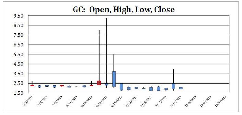
Cracks in the system started to appear on December 31, 2018 year-end. GC Repo rates opened at 2.93% and a panic ensued. Rates backed-up all the way to 7.25% before finally closing at 4.00% at 3:00 PM. It was a real eye opener. The Repo market had not seen such rate volatility in years. It was a shock. And, it was even more of a shock that the Fed did not intervene to pump cash into the market with rates so high on a year-end.
Over the next several months, the market continued to experience increased rate volatility and small rate spikes on January month-end, March quarter-end and June quarter-end. During this time, the Fed talked about a permanent RP Program, but nothing happened. The market was waving the white flag, but there was no response from the Fed.
Lehman Moment
That brings us to September and the collapse of the Repo market. Monday, September 16 was supposed to be a normal day. The market was expecting some funding pressure due to
$19 billion in net new Treasury issuance (more securities in the market)
Tax date (cash leaving the market for the Treasury)
Money Market Fund cash decreased the previous week by about $20 billion (less cash in the Repo market)
Bond market sell-off the previous week (generally adds collateral to the Repo market)
A holiday in Japan (?)
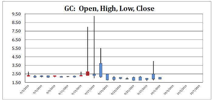
All of these factors are a normal part of the Repo market. Cash comes in and out of the market. Securities come in and out of the market. The market finds a clearing price. In fact, on September 16, the Repo GC rate opened at 2.33%. The market was expecting a little funding pressure. Nothing extraordinary. In reality, there was no Lehman moment. The only thing the Repo panic has in common with Lehman are the calendar dates.
Market Panic Dynamics
During the week of September 16, bids were thin. That is, when a bid was hit, the sellers had much more collateral to sell than the buyers (who were long cash) wanted to buy. Bids were hit and the market backed-up immediately. 3.00% traded, 3.50% traded, then 4.00%, then 4.50%, etc. The amount of securities hitting the market kept overwhelming the buyers. Everyone who was long collateral was in a rush to sell because rates were going higher. Everyone who was long cash didn’t want to buy because rates were going higher. The market peaked at 9.25%.
During the morning, as cash came into the market, rates recovered slightly. Behind the scenes it meant a cash investor had just locked-in their cash investment at a bank. The Repo trader at the bank now had actual cash to invest and they rushed to lock-in their profit. However, once that cash investment was all filled, the bids were thin again until another chunk of cash came into the market.
Look at it this way. Suppose you are a Repo trader at a large bank and your cash client calls you at 8:00 AM every day to invest their cash and set a rate. Before 8:00 AM, why lock-in a Repo rate of 3.00% at 7:30 AM when rates are gaping higher. Between 7:30 AM and 8:00 AM, there are a whole 30 more minutes for rates to keep moving higher. And 30 minutes are a long time in the Repo market at 7:30 AM! And that’s exactly what happened.
Fed Operations
On Tuesday, September 17 at 9:15 AM, during the depth of the market panic, the Fed realized they needed to inject cash into the market and announced an overnight RP operation. This was the first time the Fed used this operation in years. The operation was successful. They pumped $53.15 billion into the market and Repo GC rates closed at 2.30%; within the realm of normal. Over the next two days the Fed continued overnight operations entering the market at 8:15 AM each day and rates stabilized. On Friday, September 20, the Fed announced a schedule for overnight and term operations that went through quarterend and into October. The three term operations eventually pumped $139 billion in the market over quarter-end. On the day of quarter-end, the Fed executed a $63.5 billion overnight operation in addition to the term operations. The timing of that operation was moved up to 7:45 AM on quarter-end.
Overall, the Fed got it right. They pumped a total of $202.5 billion into the Repo market through quarter-end and progressively moved the timing of the operations from 9:15 AM to 7:45 AM. The Repo market is now functioning smoothly.
Who Won And Who Lost?
The question of who won and who lost during the Repo panic will inevitably come up. To sum it up, bank repo desks won, cash investors won, and leveraged market participants lost. Here is a closer look:
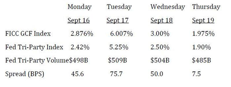
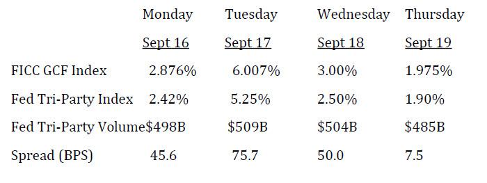
1. Bank Repo Desks – It’s pretty hard to determine exactly how much money was made or lost that week, but we can generate some rough estimates. Note: please remember there are a lot of moving parts. This is a simple estimate. If we compare the FICC GCF Index to the Fed Tri-Party Index, we can gauge, on average, where banks borrowed securities (FICC GCF) and where banks borrowed cash (Tri-Party). If we use Thursday, September 19 as a “control” date where the Street makes 7.5 basis points, we estimate that the Street normally makes about $1 million a day on Tri-Party Repo transactions. On Monday, September 16, the FICC GCF Index was 2.876% and the Tri-Party Index was 2.42% for a 45.6 basis point spread. Using the Tri-Party volume of $498 billion, means, just for Tri-Party transactions, the Street made about $6.3 million that day. The spread was even wider on Tuesday at 75.7 basis points and the profit that day was at least $10.7 million, followed by another $7 million on Wednesday. Naturally the Street marks-up clients more than the interdealer average and there is an undetermined about of deliverable GC Repo transactions, and, of course, wider spreads in the Specials market.
2. Cash Investors – Let’s say, under normal circumstances, the Tri-Party Index would be around 2.15% before the ease and at 1.90% after the ease. That means cash investors took in an additional $3.7 million in interest on Monday, $43.8 million on Tuesday, and $4.9 million on Wednesday. Thursday was a scratch. Not a bad week for cash investors! And, just like the banks, there are still a large amount of deliverable Repo GC transactions that can’t be counted.
3. Leveraged Market Participants – These are the entities that paid the price of the panic. If you add up the additional income that the banks and cash investors made, most of this came from the leveraged market participants. Based on the Tri-Party transactions, leveraged players lost, at a minimum, of $73 million that week. Once again, that figure does not include a calculation for deliverable GC Repo transactions. So … the bottom line is … I am comfortable saying that banks and cash investors earned an extra $150 million at the expense of leveraged market participants that week.
Revelations
Bank Reserves – The decline in bank reserves didn’t cause the Repo panic, but the dwindling supply of reserves could have created a smaller cushion of extra liquidity ready to enter the Repo market. In other words, the amount of excess reserves coming out of the Fed account and into the Repo market is possibly maxed out. Perhaps the bank reserves that are rate sensitive already moved out of the Fed as the IOER rate was cut. What’s left are the reserves that are not rate sensitive and therefore a one-day Repo rate spike is not enough incentive to move that liquidity out
Declining excess bank reserves might be the result of Repo market funding pressure and not the cause. Over the past year as Repo rates moved relatively higher and the Fed lowered the IOER, perhaps funds moved out of reserves into Repo just for that reason
Modern Day Bank Run – The collateral sellers (shadow banks) need funding. And they need it between 7:00 AM and 8:30 AM. The panic was a classic “run on the bank.” Cash investors did not pull cash out of the market, but they made borrowing cash more expensive. The leverage market participants had no choice but to accept prevailing rates
Price Not Credit – At no point during the Repo market panic did credit break down. The market didn’t seize up. Counterparties continued to trade. Just interest rates went higher and higher. In other words, there was never a time when there was no bid for collateral. There was always a bid. The bids just kept moving higher
Though bank balance sheets are constrained by bank regulation, banks are still the main conduit for cash investors and the Federal Reserve to inject cash into the Repo market
Question: Did the Fed solve the Repo funding problem by the size of the operations or the timing? Naturally, most traders assume it’s the dollar amount that eased the Repo panic. Maybe it’s the fact that the Fed plugged the timing mismatch between the collateral sellers and cash providers?
One question that remains unanswered is what sparked the Repo panic? I still believe a block of cash left the market and has not yet returned
Recommendations
The market was spooked by the rate spike last year-end and was hoping for a structural change after every FOMC meeting this year. It all came to a head two weeks ago. Here are some things that the Fed should or should not do to fix the Repo liquidity problem:
1. RP Program
The program would be like the RRP Program, but in reverse. Instead of injecting securities into the market like the RRP Program, the RP Program would inject cash. Sounds like a good idea. A simple solution to eliminate funding spikes. However, the RP Program is a little more complicated. Such a program can come in two forms. Philosophically, is it a rate ceiling to eliminate rate spikes, like on year-end or quarter-end? Or is it a tool to better manage overnight rates, keeping them within the target range? There are pluses and minus for both.
Rate Ceiling Facility – If the goal to prevent rate spikes, the Fed can set the RP rate 25 or 50 basis points above the upper target rate. At the current target range, the RP rate would be set at 2.25% or 2.50%. Those rates are low enough to prevent rate spikes but high enough to avoid becoming an everyday funding tool for market participants
Better Manage Rates – If the Fed wants to fine tune Repo rates, keeping them within the target range, they can set the RP rate at the upper target rate. At the current range, that would be 2.00%. With the Fed willing to inject billions of dollars of cash in the market at 2.00%, Repo rates would rarely trade above 2.00%. The drawback is that it would appear the Fed is funding leveraged market participants. Lending cash to speculators (Gasp!). Such a tight spread is probably a no-go
2. More Quantitative Easing (QE)?
QE is a monetary policy and is not a tool to provide liquidity to the Repo market. It should not be a part of managing overnight interest rates.
3. Eliminate Interest On Excess Reserves (IOER)
The Fed should continue to pay interest to banks on required reserves but stop paying interest on excess reserves. That will get more cash out of the Fed and into the market. Why should private investors (banks) receive a market rate of interest investing with the government (the Fed)? Added bonus – the Fed will no longer need to keep tweaking the IOER rate.
4. Continue RP Operations
Back a few months ago, I recommended in my Repo Market Commentary that the Fed resume RP operations instead of initiating a permanent RP Program. “Bring back the System RP!” I wrote. My recommendation stands. I don’t believe a permanent facility is needed. RP operations give the Fed flexibility – they can choose overnight or term, choose the timing, and even enter the market twice in one day if necessary. The downside is that Fed overnight and term RP operations stress Primary Dealer bank balance sheets – balance sheets that are already restricted by bank regulation. Could the Fed open the RP operations to other financial institutions? Like the RRP Program?
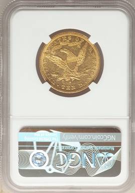
Although the 30,000-piece mintage of the 1857-O Liberty double eagle would be considered small in almost any other series, it was actually a significant increase over the production totals of the previous three years for this denomination at New Orleans. The coins were released into circulation, where they suffered heavy use and attrition over time. Despite a number of quality pieces that were recovered from the wreck of the S.S. Republic in recent times, the 1857-O is an elusive issue in AU58, and Mint State specimens are rare. This example is considerably more lustrous/brighter than seen in our images. The NGC population stands at 27 with just 7 higher.
Offered at 21,850 delivered
We do business the old fashioned way, we speak with you.
Update: Fed Chair Powell appears to have announced QE4 (but do not call it QE4!):
Discussing the liquidity shortage and repo-calypse, Powell said:
…
While a range of factors may have contributed to these developments, it is clear that without a sufficient quantity of reserves in the banking system, even routine increases in funding pressures can lead to outsized movements in money market interest rates. This volatility can impede the effective implementation of monetary policy, and we are addressing it.
Indeed, my colleagues and I will soon announce measures to add to the supply of reserves over time.
Consistent with a decision we made in January, our goal is to provide an ample supply of reserves to ensure that control of the federal funds rate and other short-term interest rates is exercised primarily by setting our administered rates and not through frequent market interventions. Of course, we will not hesitate to conduct temporary operations if needed to foster trading in the federal funds market at rates within the target range.
…
“I want to emphasize that growth of our balance sheet for reserve management purposes should in no way be confused with the large-scale asset purchase programs that we deployed after the financial crisis.
Neither the recent technical issues nor the purchases of Treasury bills we are contemplating to resolve them should materially affect the stance of monetary policy…”
Roughly translated: Don’t confuse balance sheet growth for “reserve management” with balance sheet growth for “stock market management”
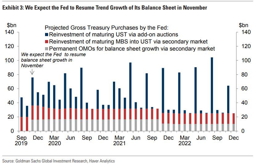
…In the chart below, Goldman summarizes its projections of the Fed’s future gross Treasury purchases. The blue bars show reinvestment of maturing UST, which occur via add-on Treasury auctions. The red bars show reinvestment of maturing MBS, which occur via the secondary market.
The grey bars are where things get fun as they show permanent OMOs to support trend growth of the Fed’s balance sheet, which will occur via intervention of the Fed’s markets desk in the secondary market.
Here, similar to Bank of America, Goldman assumes a roughly $15bn/month rate of permanent OMOs, enough to support trend growth of the balance sheet plus some additional padding over the first two years to increase the size of thebalance sheet by $150bn, restoring the reserve buffer and eliminating the current need for temporary OMOs.
That strategy would result in balance sheet growth of roughly $180bn/year and net UST purchases by the Fed (the sum of the red and grey bars) of roughly $375bn/year over the next couple of years.
And so, in just two months QE… pardon the Fed’s open market purchases of Treasurys, will return after a 5 years hiatus. Just don’t call it QE, whatever you do.
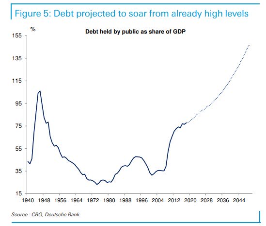
In case you wondered, here’s the real reason why The Fed found an excuse to launch QE4…
Here’s the real reason why the Fed needed any excuse to re-launch QE: someone has to buy all of this to make MMT possible in 5 years
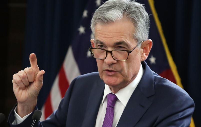
For the first time since a slew of economic data released over the past week helped ratchet up odds for another Fed rate cut in October, Fed Chairman Jerome Powell will speak Tuesday at the National Association for Business Economics’ annual meeting in Denver.
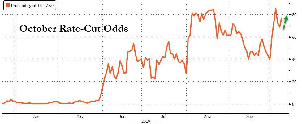
Just before Powell speaks, the odds of a rate cut in October hovered just over 75%.
Source: Bloomberg
If Powell is truly data-dependent and seeking insurance for the trade deal, then recent events suggest he will be more dovish than hawkish…
Source: Bloomberg
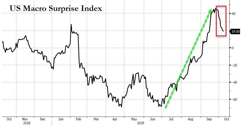
As macro data surprises begin to disappoint serially…
Source: Bloomberg
Following Powell’s prepared remarks, there will be a brief Q&A. Powell is expected to begin speaking at around 2:30 PM ET.
Powell’s comments come on the heels of Chicago Fed’s Evans’ comments that “certainly, asset valuations are quite high.”
Thank you for this opportunity to speak at the 61st annual meeting of the National Association for Business Economics.
At the Fed, we like to say that monetary policy is data dependent. We say this to emphasize that policy is never on a preset course and will change as appropriate in response to incoming information. But that does not capture the breadth and depth of what data-dependent decisionmaking means to us. From its beginnings more than a century ago, the Federal Reserve has gone to great lengths to collect and rigorously analyze the best information to make sound decisions for the public we serve.
The topic of this meeting, “Trucks and Terabytes: Integrating the ‘New’ and ‘Old’ Economies,” captures the essence of a major challenge for data-dependent policymaking. We must sort out in real time, as best we can, what the profound changes underway in the economy mean for issues such as the functioning of labor markets, the pace of productivity growth, and the forces driving inflation.
Of course, issues like these have always been with us. Indeed, 100 years ago, some of the first Fed policymakers recognized the need for more timely information on the rapidly evolving state of industry and decided to create and publish production indexes for the United States. Today I will pay tribute to the 100 years of dedicated—and often behind the scenes—work of those tracking change in the industrial landscape.
I will then turn to three challenges our dynamic economy is posing for policy at present: First, what would the consequences of a sharp rise in the price of oil be for the U.S. economy? This question, which never seems far from relevance, is again drawing our attention after recent events in the Persian Gulf. While the question is familiar, technological advances in the energy sector are rapidly changing our assessment of the answer.
Second, with terabytes of data increasingly competing with truckloads of goods in economic importance, what are the best ways to measure output and productivity? Put more provocatively, might the recent productivity slowdown be an artifact of antiquated measurement?
Third, how tight is the labor market? Given our mandate of maximum employment and price stability, this question is at the very core of our work. But answering it in real time in a dynamic economy as jobs are gained in one area but lost in others is remarkably challenging. In August, the Bureau of Labor Statistics (BLS) announced that job gains over the year through March were likely a half-million lower than previously reported. I will discuss how we are using big data to improve our grasp of the job market in the face of such revisions.
These three quite varied questions highlight the broad range of issues that currently come under the simple heading “data dependent.” After exploring them, I will comment briefly on recent developments in money markets and on monetary policy.
A Century of Industrial Production
Our story of data dependence in the face of change begins when the Fed opened for business in 1914. World War I was breaking out in Europe, and over the next four years the war would fuel profound growth and transformation in the U.S. economy.1 But you could not have seen this change in the gross national product data; the Department of Commerce did not publish those until 1942. The Census Bureau had been running a census of manufactures since 1905, but that came only every five years—an eternity in the rapidly changing economy. In need of more timely information, the Fed began creating and publishing a series of industrial output reports that soon evolved into industrial production indexes.2 The indexes initially comprised 22 basic commodities, chosen in part because they covered the major industrial groups, but also for the practical reason that data were available with less than a one-month lag. The Fed’s efforts were among the earliest in creating timely measures of aggregate production. Over the century of its existence, our industrial production team has remained at the frontier of economic measurement, using the most advanced techniques to monitor U.S. industry and nimbly track changes in production.
What Are the Consequences of an Oil Price Spike?
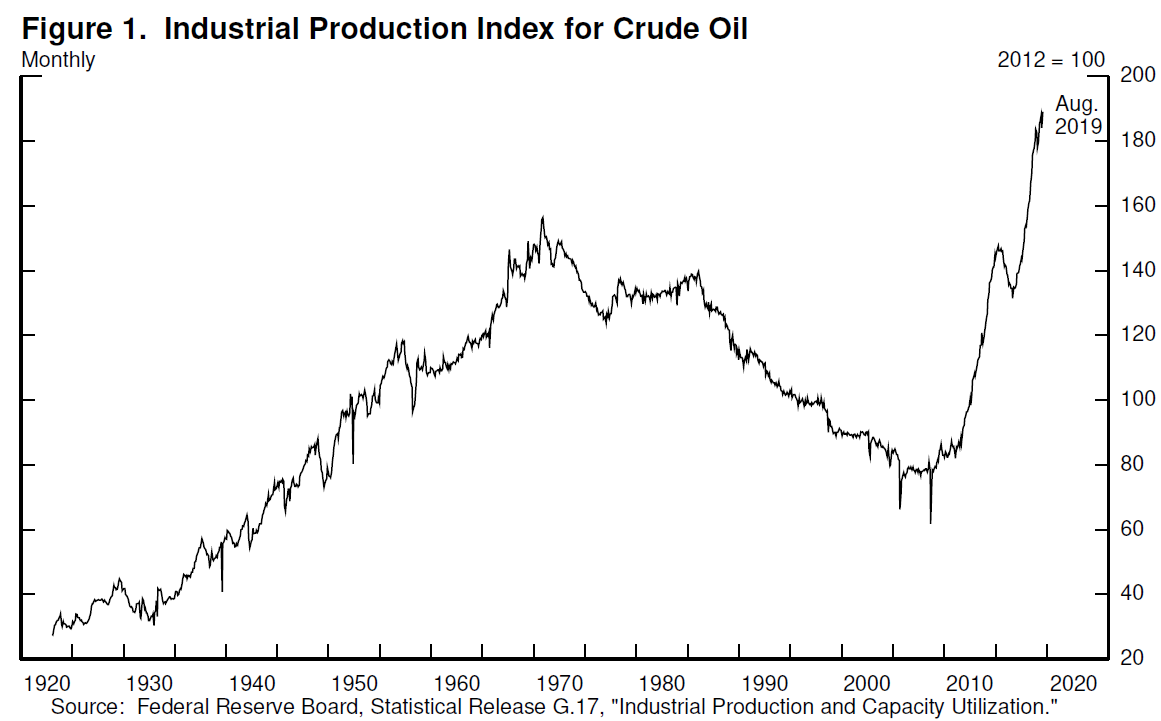
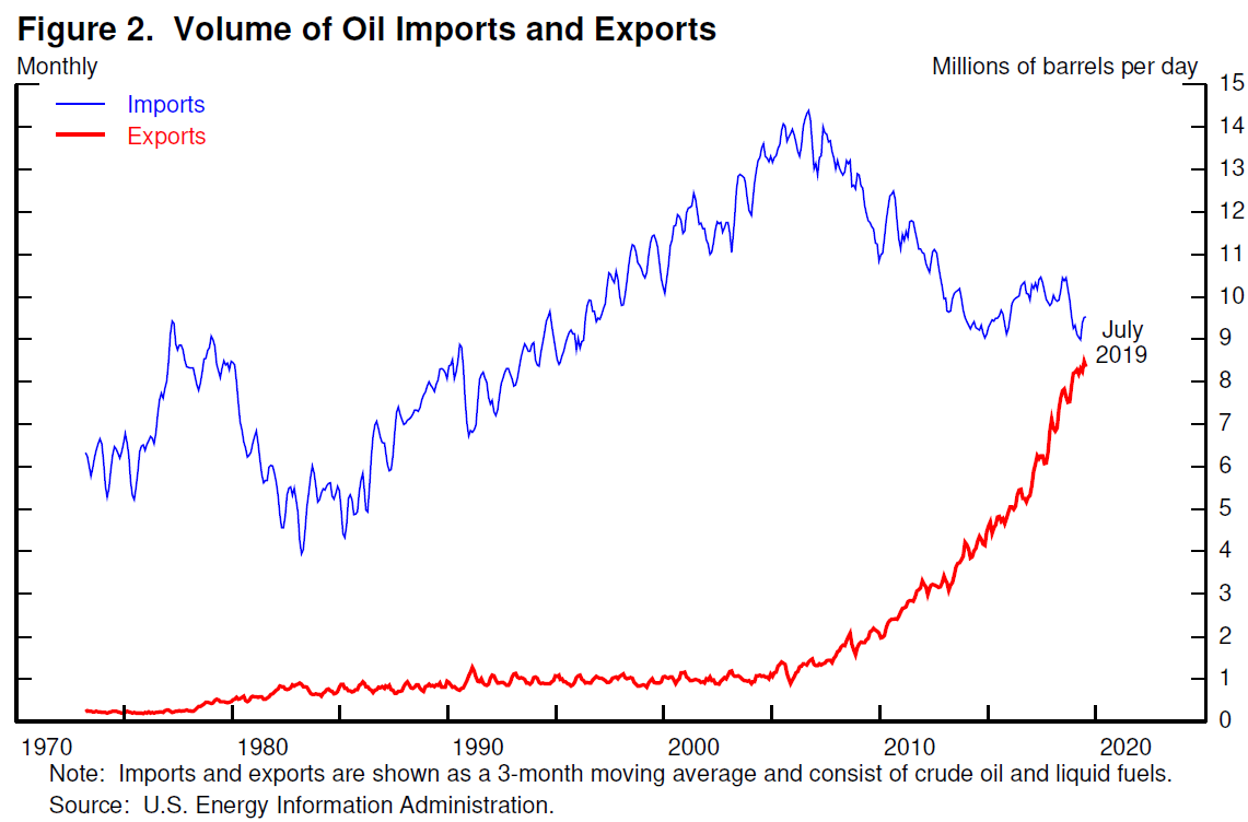
Let’s turn now to the first question of the consequences of an oil price spike. Figure 1 shows U.S. oil production since 1920. After rising fairly steadily through the early 1970s, production began a long period of gradual decline. By 2005, production was at about the same level as it had been 50 years earlier. Since then, remarkable advances in the technology for finding and extracting oil have led to a rapid increase in production to levels higher than ever before.3 In 2018, the United States became the world’s largest oil producer.4 Oil exports have surged, imports have fallen (figure 2), and the U.S. Energy Information Administration projects that this month, for the first time in many decades, the United States will be a net exporter of oil.5
As monetary policymakers, we closely monitor developments in oil markets because disruptions in these markets have played a role in several U.S. recessions and in the Great Inflation of the 1960s and 1970s. Traditionally, we assessed that a sharp rise in the price of oil would have a strong negative effect on consumers and businesses and, hence, on the U.S. economy. Today a higher oil price would still cause dislocations and hardship for many, but with exports and imports nearly balanced, the higher price paid by consumers is roughly offset by higher earnings of workers and firms in the U.S. oil industry. Moreover, because it is now easier to ramp up oil production, a sustained price rise can quickly boost output, providing a shock absorber in the face of supply disruptions. Thus, setting aside the effects of geopolitical uncertainty that may accompany higher oil prices, we now judge that a price spike would likely have nearly offsetting effects on U.S. gross domestic product (GDP).
How Should We Measure Output and Productivity?
Let’s now turn to the second question of how to best measure output and productivity. While there are some subtleties in measuring oil output, we know how to count barrels of oil. Measuring the overall level of goods and services produced in the economy is fundamentally messier, because it requires adding apples and oranges—and automobiles and myriad other goods and services. The hard-working statisticians creating the official statistics regularly adapt the data sources and methods so that, insofar as possible, the measured data provide accurate indicators of the state of the economy. Periods of rapid change present particular challenges, and it can take time for the measurement system to adapt to fully and accurately reflect the changes in the economy.
The advance of technology has long presented measurement challenges. In 1987, Nobel Prize–winning economist Robert Solow quipped that “you can see the computer age everywhere but in the productivity statistics.”6 In the second half of the 1990s, this measurement puzzle was at the heart of monetary policymaking.7 Chairman Alan Greenspan famously argued that the United States was experiencing the dawn of a new economy, and that potential and actual output were likely understated in official statistics. Where others saw capacity constraints and incipient inflation, Greenspan saw a productivity boom that would leave room for very low unemployment without inflation pressures. In light of the uncertainty it faced, the Federal Open Market Committee (FOMC) judged that the appropriate risk‑management approach called for refraining from interest rate increases unless and until there were clearer signs of rising inflation. Under this policy, unemployment fell near record lows without rising inflation, and later revisions to GDP measurement showed appreciably faster productivity growth.8
This episode illustrates a key challenge to making data-dependent policy in real time: Good decisions require good data, but the data in hand are seldom as good as we would like. Sound decisionmaking therefore requires the application of good judgment and a healthy dose of risk management.
Productivity is again presenting a puzzle. Official statistics currently show productivity growth slowing significantly in recent years, with the growth in output per hour worked falling from more than 3 percent a year from 1995 to 2003 to less than half that pace since then.9 Analysts are actively debating three alternative explanations for this apparent slowdown: First, the slowdown may be real and may persist indefinitely as productivity growth returns to more‑normal levels after a brief golden age.10 Second, the slowdown may instead be a pause of the sort that often accompanies fundamental technological change, so that productivity gains from recent technology advances will appear over time as society adjusts.11 Third, the slowdown may be overstated, perhaps greatly, because of measurement issues akin to those at work in the 1990s.12 At this point, we cannot know which of these views may gain widespread acceptance, and monetary policy will play no significant role in how this puzzle is resolved. As in the late 1990s, however, we are carefully assessing the implications of possibly mismeasured productivity gains. Moreover, productivity growth seems to have moved up over the past year after a long period at very low levels; we do not know whether that welcome trend will be sustained.
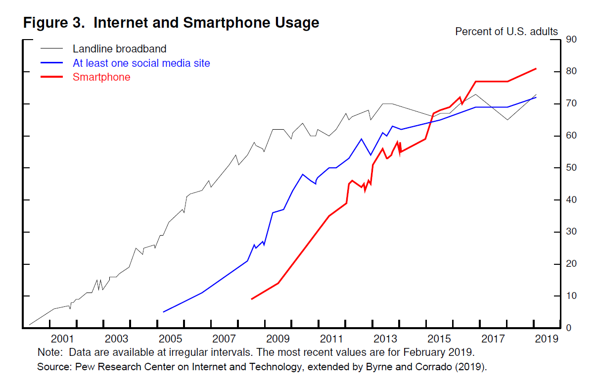
Recent research suggests that current official statistics may understate productivity growth by missing a significant part of the growing value we derive from fast internet connections and smartphones. These technologies, which were just emerging 15 years ago, are now ubiquitous (figure 3). We can now be constantly connected to the accumulated knowledge of humankind and receive near instantaneous updates on the lives of friends far and wide. And, adding to the measurement challenge, many of these services are free, which is to say, not explicitly priced. How should we value the luxury of never needing to ask for directions? Or the peace and tranquility afforded by speedy resolution of those contentious arguments over the trivia of the moment?
Researchers have tried to answer these questions in various ways.13 For example, Fed researchers have recently proposed a novel approach to measuring the value of services consumers derive from cellphones and other devices based on the volume of data flowing over those connections.14 Taking their accounting at face value, GDP growth would have been about 1/2 percentage point higher since 2007, which is an appreciable change and would be very good news. Growth over the previous couple of decades would also have been about 1/4 percentage point higher as well, implying that measurement issues of this sort likely account for only part of the productivity slowdown in current statistics. Research in this area is at an early stage, but this example illustrates the depth of analysis supporting our data-dependent decisionmaking.
How Tight Is the Labor Market?
Let me now turn from the measurement issues raised by the information age to an issue that has long been at the center of monetary policymaking: How tight is the labor market? Answering this question is central to our outlook for both of our dual-mandate goals of maximum employment and price stability. While this topic is always front and center in our thinking, I am raising it today to illustrate how we are using big data to inform policymaking.
Until recently, the official data showed job gains over the year through March 2019 of about 210,000 a month, which is far higher than necessary to absorb new entrants into the labor force and thus hold the unemployment rate constant. In August, the BLS publicly previewed the benchmark data revision coming in February 2020, and the news was that job gains over this period were more like 170,000 per month—a meaningfully lower number that itself remains subject to revision. The pace of job gains is hard to pin down in real time largely because of the dynamism of our economy: Many new businesses open and others close every month, creating some jobs and ending others, and definitive data on this turnover arrive with a substantial lag. Thus, initial data are, in part, sophisticated guesses based on what is known as the birth–death model of firms.
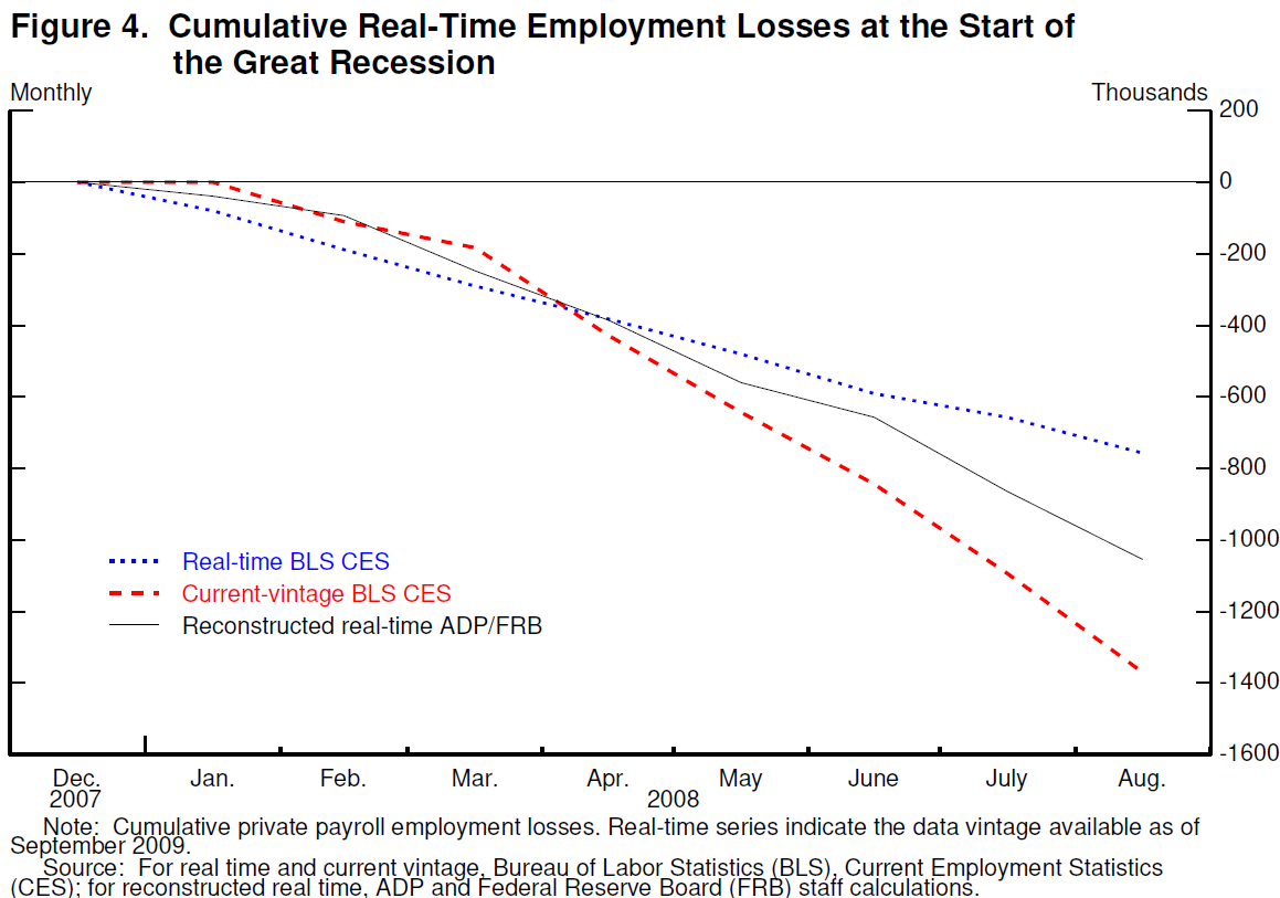
Several years ago, we began a collaboration with the payroll processing firm ADP to construct a measure of payroll employment from their data set, which covers about 20 percent of the nation’s private workforce and is available to us with a roughly one-week delay.15 As described in a recent research paper, we constructed a measure that provides an independent read on payroll employment that complements the official statistics.16 While experience is still limited with the new measure, we find promising evidence that it can refine our real-time picture of job gains. For example, in the first eight months of 2008, as the Great Recession was getting underway, the official monthly employment data showed total job losses of about 750,000 (figure 4). A later benchmark revision told a much bleaker story, with declines of about 1.5 million. Our new measure, had it been available in 2008, would have been much closer to the revised data, alerting us that the job situation might be considerably worse than the official data suggested.17
We believe that the new measure may help us better understand job market conditions in real time. The preview of the BLS benchmark revision leaves average job gains over the year through March solidly above the pace required to accommodate growth in the workforce over that time, but where we had seen a booming job market, we now see more-moderate growth. The benchmark revision will not directly affect data for job gains since March, but experience with past revisions suggests that some part of the benchmark will likely carry forward. Thus, the currently reported job gains of 157,000 per month on average over the past three months may well be revised somewhat lower. Based on a range of data and analysis, including our new measure, we now judge that, even allowing for such a revision, job gains remain above the level required to provide jobs for new entrants to the jobs market over time. Of course, the pace of job gains is only one of many job market issues that figure into our assessment of how the economy is performing relative to our maximum-employment mandate and our assessment of any inflationary pressures arising in the job market.
What Does Data Dependence Mean at Present?
In summary, data dependence is, and always has been, at the heart of policymaking at the Federal Reserve. We are always seeking out new and better sources of information and refining our analysis of that information to keep us abreast of conditions as our economy constantly reinvents itself. Before wrapping up, I will discuss recent developments in money markets and the current stance of monetary policy.
Our influence on the financial conditions that affect employment and inflation is indirect. The Federal Reserve sets two overnight interest rates: the interest rate paid on banks’ reserve balances and the rate on our reverse repurchase agreements. We use these two administered rates to keep a market-determined rate, the federal funds rate, within a target range set by the FOMC. We rely on financial markets to transmit these rates through a variety of channels to the rates paid by households and businesses—and to financial conditions more broadly.
In mid-September, an important channel in the transmission process—wholesale funding markets—exhibited unexpectedly intense volatility. Payments to meet corporate tax obligations and to purchase Treasury securities triggered notable liquidity pressures in money markets. Overnight interest rates spiked, and the effective federal funds rate briefly moved above the FOMC’s target range. To counter these pressures, we began conducting temporary open market operations. These operations have kept the federal funds rate in the target range and alleviated money market strains more generally.
While a range of factors may have contributed to these developments, it is clear that without a sufficient quantity of reserves in the banking system, even routine increases in funding pressures can lead to outsized movements in money market interest rates. This volatility can impede the effective implementation of monetary policy, and we are addressing it. Indeed, my colleagues and I will soon announce measures to add to the supply of reserves over time. Consistent with a decision we made in January, our goal is to provide an ample supply of reserves to ensure that control of the federal funds rate and other short-term interest rates is exercised primarily by setting our administered rates and not through frequent market interventions. Of course, we will not hesitate to conduct temporary operations if needed to foster trading in the federal funds market at rates within the target range.
Reserve balances are one among several items on the liability side of the Federal Reserve’s balance sheet, and demand for these liabilities—notably, currency in circulation—grows over time. Hence, increasing the supply of reserves or even maintaining a given level over time requires us to increase the size of our balance sheet. As we indicated in our March statement on balance sheet normalization, at some point, we will begin increasing our securities holdings to maintain an appropriate level of reserves.18 That time is now upon us.
I want to emphasize that growth of our balance sheet for reserve management purposes should in no way be confused with the large-scale asset purchase programs that we deployed after the financial crisis. Neither the recent technical issues nor the purchases of Treasury bills we are contemplating to resolve them should materially affect the stance of monetary policy, to which I now turn.
Our goal in monetary policy is to promote maximum employment and stable prices, which we interpret as inflation running closely around our symmetric 2 percent objective. At present, the jobs and inflation pictures are favorable. Many indicators show a historically strong labor market, with solid job gains, the unemployment rate at half-century lows, and rising prime-age labor force participation. Wages are rising, especially for those with lower-paying jobs. Inflation is somewhat below our symmetric 2 percent objective but has been gradually firming over the past few months. FOMC participants continue to see a sustained expansion of economic activity, strong labor market conditions, and inflation near our symmetric 2 percent objective as most likely. Many outside forecasters agree.
But there are risks to this favorable outlook, principally from global developments. Growth around much of the world has weakened over the past year and a half, and uncertainties around trade, Brexit, and other issues pose risks to the outlook. As those factors have evolved, my colleagues and I have shifted our views about appropriate monetary policy toward a lower path for the federal funds rate and have lowered its target range by 50 basis points. We believe that our policy actions are providing support for the outlook. Looking ahead, policy is not on a preset course. The next FOMC meeting is several weeks away, and we will be carefully monitoring incoming information. We will be data dependent, assessing the outlook and risks to the outlook on a meeting-by-meeting basis. Taking all that into account, we will act as appropriate to support continued growth, a strong job market, and inflation moving back to our symmetric 2 percent objective.
Courtesy of ZeroHedge by Tyler DurdenFri, 10/04/2019 – 14:01
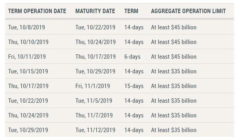
Anyone who expected that the easing of the quarter-end funding squeeze in the repo market would mean the Fed would gradually fade its interventions in the repo market, was disappointed on Friday afternoon when the NY Fed announced it would extend the duration of overnight repo operations (with a total size of $75BN) for at least another month, while also offer no less than eight 2-week term repo operations until November 4, 2019, which confirms that the funding unlocked via term repo is no longer merely a part of the quarter-end arsenal but an integral part of the Fed’s overall “temporary” open market operations… which are starting to look quite permanent.
This is the statement published moments ago by the NY Fed:
In accordance with the most recent Federal Open Market Committee (FOMC) directive, the Open Market Trading Desk (the Desk) at the Federal Reserve Bank of New York will conduct a series of overnight and term repurchase agreement (repo) operations to help maintain the federal funds rate within the target range.
Effective the week of October 7, the Desk will offer term repos through the end of October as indicated in the schedule below. The Desk will continue to offer daily overnight repos for an aggregate amount of at least $75 billion each through Monday, November 4, 2019.
Securities eligible as collateral include Treasury, agency debt, and agency mortgage-backed securities. Awarded amounts may be less than the amount offered, depending on the total quantity of eligible propositions submitted. Additional details about the operations will be released each afternoon for the following day’s operation(s) on the Repurchase Agreement Operational Details webpage. The operation schedule and parameters are subject to change if market conditions warrant or should the FOMC alter its guidance to the Desk.
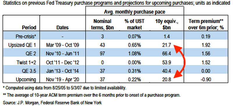
What this means is that until such time as the Fed launches Permanent Open Market Operations – either at the November or December FOMC meeting, which according to JPMorgan will be roughly $37BN per month, or approximately the same size as QE1…
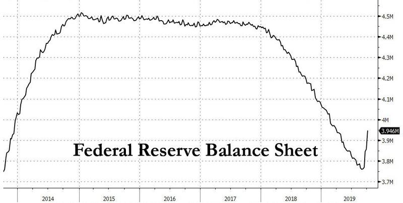
… the NY Fed will continue to inject liquidity via the now standard TOMOs: overnight and term repos. At that point, watch as the Fed’s balance sheet, which rose by $185BN in the past month, continues rising indefinitely as QE4 is quietly launched to no fanfare.
The 3 and 9 in the date are noticeably recut north on this variety, one of the scarcer varieties for the issue. Doug Winter estimates as many as 300 to 400 examples survive from a mintage of 18,140 coins, although the population thins considerably in the upper AU range, and true Mint State coins are rare.
Offered at $7,475 delivered
We do business the old fashioned way, we speak with you.

